Centrality (중심성: 개인(node)의 위치가 전체에서 어디를 차지하는가? 얼마나 중요한가?) vs.
Centralization (중앙(화)성: 얼마나 뭉쳐져 있는가?)

# Social Network Analysis: Closeness Centrality  
library(sna)

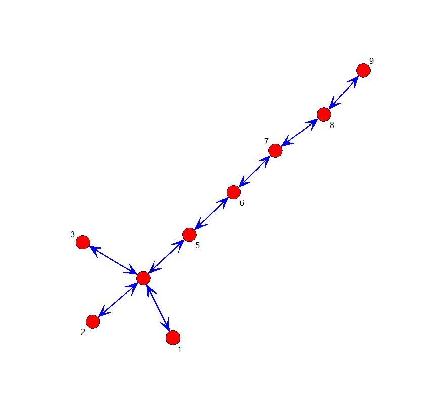
# The nearly linear network
L <- matrix(c(0,0,0,1,0,0,0,0,0,
              0,0,0,1,0,0,0,0,0,
              0,0,0,1,0,0,0,0,0,
              1,1,1,0,1,0,0,0,0,
              0,0,0,1,0,1,0,0,0,
              0,0,0,0,1,0,1,0,0,
              0,0,0,0,0,1,0,1,0,
              0,0,0,0,0,0,1,0,1,
              0,0,0,0,0,0,0,1,0),byrow=T,nrow=9)

gplot(L, displaylabels = T, vertex.cex = 1, label.cex = 2, edge.col="red", 
             boxed.labels = F, arrowhead.cex = 1, mode = "kamadakawai")

Node 1 은 다른 node와 얼마나 가까운가?
= sum of geodesic distance to others / n
= (2 + 2 + 1 + 2 + 3 + 4 + 5 + 6) / 8 = 25 / 8 의 역수
⇒ 8 / 25 = 0.32

Node 4 은 다른 node들과 얼마나 가까운가?
= sum of geodesic distance to others / n
= (1 + 1 + 1 + 1 + 2 + 3 + 4 + 5) / 8 = 18 / 8 의 역수 (가까운 거리의 합이 작으므로 이를 크게 하기 위해서)
⇒ 8 / 18 = 0.44

Node 1 과 Node 4 중 어느 것이 중심성이 높은가?

위의 방법으로 각 노드의 중심성 (closesness) 구하기:

round(closeness(L),2) # Type 1 closeness
[1] 0.32 0.32 0.32 0.44 0.47 0.44 0.38 0.31 0.24

다른 방법의 closesness

round(closeness(L,cmode="suminvundir"),2) # Type 2 closeness
[1] 0.43 0.43 0.43 0.66 0.57 0.54 0.51 0.46 0.35

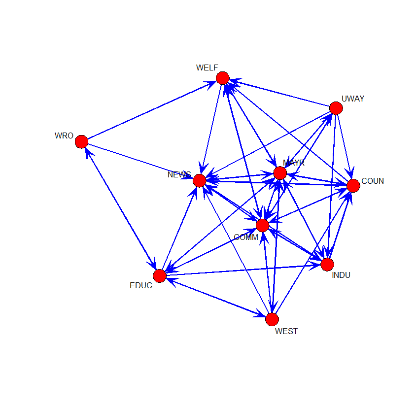
# Knoke's information network (Hanneman and Riddle, 2005)
knoke.infor <- as.matrix(read.table("knoke-infor.txt",header=T))
rownames(knoke.infor) <- colnames(knoke.infor)
gplot(knoke.infor, displaylabels=T, vertex.cex=2, edge.col="blue", boxed.labels=F, arrowhead.cex=1.25)

1. COUN: county government
2. COMM: chamber of commerce
3. EDUC: board of education
4. INDU: Industry development agency
5. MAYR: Mayor
6. WRO: Women Right Organization group
7. NEWS: Newspaper
8. WAY: United Way (private organization)
9. WELF: Welfare
10. WEST: West group (private organization)

round(closeness(knoke.infor,cmode="suminvdir"),2)
 [1] 0.70 0.89 0.83 0.70 0.94 0.63 0.65 0.81 0.65 0.78

round(closeness(t(knoke.infor),cmode="suminvdir"),2)
 [1] 0.76 0.94 0.72 0.78 0.94 0.46 1.00 0.59 0.78 0.61

노드 k에 대해서 노드 i 과 j 의 최단 경로 사이에 끼이게 되는 경우의 총합

# Social Network Analysis: Betweenness Centrality 
library(sna)

# The nearly linear network
L <- matrix(c(0,0,0,1,0,0,0,0,0,
              0,0,0,1,0,0,0,0,0,
              0,0,0,1,0,0,0,0,0,
              1,1,1,0,1,0,0,0,0,
              0,0,0,1,0,1,0,0,0,
              0,0,0,0,1,0,1,0,0,
              0,0,0,0,0,1,0,1,0,
              0,0,0,0,0,0,1,0,1,
              0,0,0,0,0,0,0,1,0),byrow=T,nrow=9)
gplot(L, displaylabels=T, vertex.cex=1, label.cex=1, 
      edge.col="red", boxed.labels=F, arrowhead.cex=1, 
      mode="kamadakawai")

</code>betweenness(L)
</code>

[1]  0  0  0 36 32 30 24 14  0

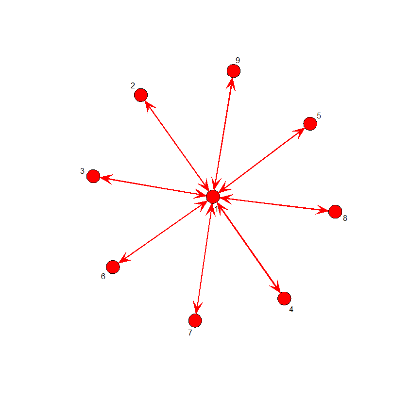
# The star network
S <- matrix(c(0,1,1,1,1,1,1,1,1,
              1,0,0,0,0,0,0,0,0,
              1,0,0,0,0,0,0,0,0,
              1,0,0,0,0,0,0,0,0,
              1,0,0,0,0,0,0,0,0,
              1,0,0,0,0,0,0,0,0,
              1,0,0,0,0,0,0,0,0,
              1,0,0,0,0,0,0,0,0,
              1,0,0,0,0,0,0,0,0),byrow=T,nrow=9)
gplot(S, displaylabels=T, vertex.cex=1, label.cex=1, 
      edge.col="red", boxed.labels=F, arrowhead.cex=1, 
      mode="kamadakawai")

betweenness(S)

[1] 56  0  0  0  0  0  0  0  0

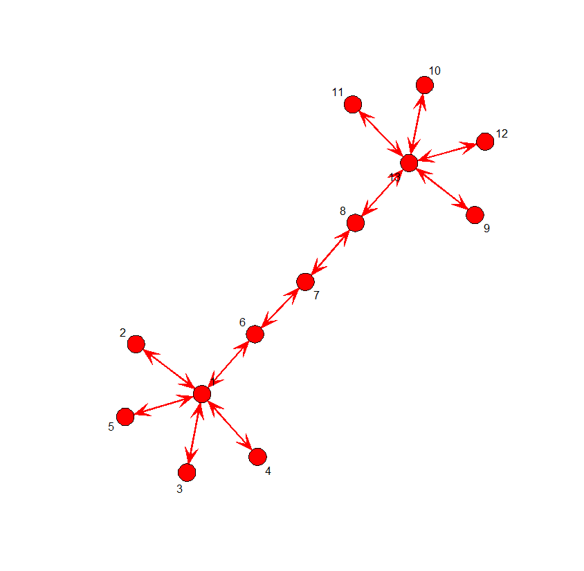
# Two stars network
twostars <- matrix(0,13,13)
edges <- matrix(c(1,2,1,3,1,4,1,5,1,6,
                  6,7,7,8,8,13,9,13,10,13,11,13,12,13),
                  byrow=T,ncol=2)
twostars[edges] <- 1
twostars <- twostars + t(twostars) - twostars * t(twostars)

gplot(twostars, displaylabels=T, vertex.cex=1, label.cex=1, 
      edge.col="red", boxed.labels=F, arrowhead.cex=1, mode="kamadakawai")
betweenness(twostars)
closeness(twostars)

>> betweenness(twostars)
 [1] 76  0  0  0  0 70 72 70  0  0  0  0 76
> round(closeness(twostars),2)
 [1] 0.35 0.27 0.27 0.27 0.27 0.39 0.40 0.39 0.27 0.27 0.27 0.27 0.35